Test Logistic Regression Model

HYPOTHESIS

I am using the Gapminder data set. My Response variable is Polity Score. I am testing if political stand of a country has an association with Internet usage. Other explanatory variables considered are – female employment rate, percentage population in armed forces, life expectancy and employment rate of a country. The hypothesis is that a country tends to have an opinion, either autocratic or democratic, where internet use rate is more. Hence I am expecting a positive intercept

CODE

# -*- coding: utf-8 -*-
"""
Created on Tue Dec 22 12:38:05 2015

@author: Abhishek
"""

import numpy
import pandas
import statsmodels.api as sm
import seaborn
import statsmodels.formula.api as smf 

# bug fix for display formats to avoid run time errors
pandas.set_option('display.float_format', lambda x: '%f'%x)

data = pandas.read_csv('gapminder.csv', low_memory=False)

# Replace empty values with NaN
data['polityscore'] = data['polityscore'].astype(numpy.object)
data['polityscore'] = data['polityscore'].replace(' ',numpy.nan)
data['polityscore'] = data['polityscore'].replace('',numpy.nan)

data['femaleemployrate'] = data['femaleemployrate'].astype(numpy.object)
data['femaleemployrate'] = data['femaleemployrate'].replace(' ',numpy.nan)
data['femaleemployrate'] = data['femaleemployrate'].replace('',numpy.nan)

data['internetuserate'] = data['internetuserate'].astype(numpy.object)
data['internetuserate'] = data['internetuserate'].replace(' ',numpy.nan)
data['internetuserate'] = data['internetuserate'].replace('',numpy.nan)

data['armedforcesrate'] = data['armedforcesrate'].astype(numpy.object)
data['armedforcesrate'] = data['armedforcesrate'].replace(' ',numpy.nan)
data['armedforcesrate'] = data['armedforcesrate'].replace('',numpy.nan)

data['lifeexpectancy'] = data['lifeexpectancy'].astype(numpy.object)
data['lifeexpectancy'] = data['lifeexpectancy'].replace(' ',numpy.nan)
data['lifeexpectancy'] = data['lifeexpectancy'].replace('',numpy.nan)

data['employrate'] = data['employrate'].astype(numpy.object)
data['employrate'] = data['employrate'].replace(' ',numpy.nan)
data['employrate'] = data['employrate'].replace('',numpy.nan)

data['incomeperperson'] = data['incomeperperson'].astype(numpy.object)
data['incomeperperson'] = data['incomeperperson'].replace('',numpy.nan)
data['incomeperperson'] = data['incomeperperson'].replace(' ',numpy.nan)


# Response Variable
data['polityscore'] = pandas.to_numeric(data['polityscore'], errors='coerce')

# Explanatory Variables
data['incomeperperson'] = pandas.to_numeric(data['incomeperperson'], errors='coerce')
data['employrate'] = pandas.to_numeric(data['employrate'], errors='coerce')
data['femaleemployrate'] = pandas.to_numeric(data['femaleemployrate'], errors='coerce')
data['internetuserate'] = pandas.to_numeric(data['internetuserate'], errors='coerce')
data['armedforcesrate'] = pandas.to_numeric(data['armedforcesrate'], errors='coerce')
data['lifeexpectancy'] = pandas.to_numeric(data['lifeexpectancy'], errors='coerce')

sub1 = data.copy()

#%%
# Data Management: Polity Score is chosen as the response variable. 
# -10 to -5: Autocratic, -5 to 5: Anocratic and 5 to 10: Democratic
# Here, Anocratic countries are coded as 0 and countries with political 
# biases are coded as 1. Hence we have out bivariate response variable

def RecodePolityScore (row):
   if row['polityscore']<=-5 or row['polityscore']>=5 :
      return 1
   elif row['polityscore']>-5 and row['polityscore']<5 data-blogger-escaped-0="" data-blogger-escaped-:="" data-blogger-escaped-and="" data-blogger-escaped-def="" data-blogger-escaped-elif="" data-blogger-escaped-femaleemployrate="" data-blogger-escaped-if="" data-blogger-escaped-numpy.nan="" data-blogger-escaped-recodefemaleemprate="" data-blogger-escaped-return="" data-blogger-escaped-row="">=65 and row['femaleemployrate'] != numpy.nan :
      return 1

def RecodeInternetUseRate (row):
   if row['internetuserate']<=10 and row['internetuserate'] != numpy.nan:
      return 0
   elif row['internetuserate']>=65 and row['internetuserate'] != numpy.nan:
      return 1

def RecodeArmedForcesRate (row):
   if row['armedforcesrate']<=1 and row['armedforcesrate'] != numpy.nan:
      return 0
   elif row['armedforcesrate']>=5 and row['armedforcesrate'] != numpy.nan:
      return 1

def RecodeLifeExpectancyRate (row):
   if row['lifeexpectancy']<=55 and row['lifeexpectancy'] != numpy.nan :
      return 0
   elif row['lifeexpectancy']>=80 and row['lifeexpectancy'] != numpy.nan :
      return 1

def RecodeEmploymentRate (row):
   if row['employrate']<=45 and row['employrate'] != numpy.nan :
      return 0
   elif row['employrate']>=75 and row['employrate'] != numpy.nan :
      return 1

def RecodeIncomePerPerson (row):
   if row['incomeperperson']<=250 and row['incomeperperson'] != numpy.nan :
      return 0
   elif row['incomeperperson']>=10000 and row['incomeperperson'] != numpy.nan :
      return 1

# Check that recoding is done      
sub1['polityscore'] = sub1.apply(lambda row: RecodePolityScore(row),axis=1)
chk1d = sub1['polityscore'].value_counts(sort=False, dropna=True)
print (chk1d)

sub1['femaleemployrate'] = sub1.apply(lambda row: RecodeFemaleEmpRate(row),axis=1)
chk1d = sub1['femaleemployrate'].value_counts(sort=False, dropna=True)
print (chk1d)

sub1['internetuserate'] = sub1.apply(lambda row: RecodeInternetUseRate(row),axis=1)
chk1d = sub1['internetuserate'].value_counts(sort=False, dropna=True)
print (chk1d)

sub1['armedforcesrate'] = sub1.apply(lambda row: RecodeArmedForcesRate(row),axis=1)
chk1d = sub1['armedforcesrate'].value_counts(sort=False, dropna=True)
print (chk1d)

sub1['lifeexpectancy'] = sub1.apply(lambda row: RecodeLifeExpectancyRate(row),axis=1)
chk1d = sub1['lifeexpectancy'].value_counts(sort=False, dropna=True)
print (chk1d)

sub1['employrate'] = sub1.apply(lambda row: RecodeEmploymentRate(row),axis=1)
chk1d = sub1['employrate'].value_counts(sort=False, dropna=True)
print (chk1d)

sub1['incomeperperson'] = sub1.apply(lambda row: RecodeIncomePerPerson(row),axis=1)
chk1d = sub1['incomeperperson'].value_counts(sort=False, dropna=True)
print (chk1d)


#%%
# Logistic Regression

lreg1 = smf.logit(formula = 'polityscore ~ internetuserate', data = sub1).fit()
print(lreg1.summary())
print()

# Odds Ratio
print("Odds Ratio")
print("----------")
print(numpy.exp(lreg1.params))
print()

# Confidence Interval
print("Confidence Interval")
print("-------------------")
params = lreg1.params
conf = lreg1.conf_int()
conf['OR'] = params
conf.columns = ['Lower CI', 'Upper CI', 'OR']
print(numpy.exp(conf))

#%%
# Logistic Regression - femaleemployrate as explanatory variable

lreg2 = smf.logit(formula = 'polityscore ~ femaleemployrate', data = sub1).fit()
print(lreg2.summary())
print()

# Odds Ratio
print("Odds Ratio")
print("----------")
print(numpy.exp(lreg2.params))
print()

# Confidence Interval
print("Confidence Interval")
print("-------------------")
params = lreg2.params
conf = lreg2.conf_int()
conf['OR'] = params
conf.columns = ['Lower CI', 'Upper CI', 'OR']
print(numpy.exp(conf))

#%%
# Logistic Regression - armedforcesrate as explanatory variable

lreg3 = smf.logit(formula = 'polityscore ~ armedforcesrate', data = sub1).fit()
print(lreg3.summary())
print()

# Odds Ratio
print("Odds Ratio")
print("----------")
print(numpy.exp(lreg3.params))
print()

# Confidence Interval
print("Confidence Interval")
print("-------------------")
params = lreg3.params
conf = lreg3.conf_int()
conf['OR'] = params
conf.columns = ['Lower CI', 'Upper CI', 'OR']
print(numpy.exp(conf))

#%%
# Logistic Regression - lifeexpectancy as explanatory variable

lreg4 = smf.logit(formula = 'polityscore ~ lifeexpectancy', data = sub1).fit()
print(lreg4.summary())
print()

# Odds Ratio
print("Odds Ratio")
print("----------")
print(numpy.exp(lreg4.params))
print()

# Confidence Interval
print("Confidence Interval")
print("-------------------")
params = lreg4.params
conf = lreg4.conf_int()
conf['OR'] = params
conf.columns = ['Lower CI', 'Upper CI', 'OR']
print(numpy.exp(conf))

#%%
# Logistic Regression - employrate as explanatory variable

lreg3 = smf.logit(formula = 'polityscore ~ employrate', data = sub1).fit()
print(lreg3.summary())
print()

# Odds Ratio
print("Odds Ratio")
print("----------")
print(numpy.exp(lreg3.params))
print()

# Confidence Interval
print("Confidence Interval")
print("-------------------")
params = lreg3.params
conf = lreg3.conf_int()
conf['OR'] = params
conf.columns = ['Lower CI', 'Upper CI', 'OR']
print(numpy.exp(conf))

#%%
# Logistic Regression - incomeperperson as explanatory variable

lreg3 = smf.logit(formula = 'polityscore ~ incomeperperson', data = sub1).fit()
print(lreg3.summary())
print()

# Odds Ratio
print("Odds Ratio")
print("----------")
print(numpy.exp(lreg3.params))
print()

# Confidence Interval
print("Confidence Interval")
print("-------------------")
params = lreg3.params
conf = lreg3.conf_int()
conf['OR'] = params
conf.columns = ['Lower CI', 'Upper CI', 'OR']
print(numpy.exp(conf))

#%%
# Test of Confounding -  internetuserate + lifeexpectancy

lreg3 = smf.logit(formula = 'polityscore ~ lifeexpectancy + internetuserate', data = sub1).fit()
print(lreg3.summary())
print()

# Odds Ratio
print("Odds Ratio")
print("----------")
print(numpy.exp(lreg3.params))
print()

# Confidence Interval
print("Confidence Interval")
print("-------------------")
params = lreg3.params
conf = lreg3.conf_int()
conf['OR'] = params
conf.columns = ['Lower CI', 'Upper CI', 'OR']
print(numpy.exp(conf))

DATA MANAGEMENT

I am using the Gapminder data set where all fields are continuous quantitative. I had to bin the response and explanatory variable into 0 and 1.

• Since I am interested in whether a country is autocratic or democratic, polity score of a country has been re-coded as 1 if score falls between -10 to -5 and 5 to 10. Anocratic countries are neutral and their score falls between -5 to 5. They are recoded as 0
  
• For all explanatory variables, the 2 bins are some percentage of lowest and highest quartile.
  
  
  
  
  
  
  
  
  
  
  
  
  
  
  
  
  
  
  
• I have taken the liberty of assigning 0 and I appropriately looking at the span of values for each explanatory variable. More research into the context, that is how data was collected and what makes sense socially need to be looked into, to correctly bin the values of the explanatory variables

LOGISTIC REGRESSION

Explanatory Variable: Internet Use Rate

P Value: The parameter estimates from the table above shows that the regression is significant with p value 0.005. A linear equation will not make sense here so we move on to generating odds ratio

Odds Ratio: I can interpret the odds ratio results as, countries with high internet use rate or greater than 65% are 19.7 times more likely have a political stand (autocratic or democratic) than countries with less internet use rate or less than 10%

Confidence Interval: I can interpret the confidence interval as, there is a 95% certainty that the true population odds ratio falls between 2.46 and 157.6

Regression Analysis for all other explanatory variables

From the above results we see that income per person or GDP per capita and life expectancy are the only 2 variables who have a significant regression against polity score.

For Explanatory Variable: Income Per Person / GDP per capita

P Value: A p value of 0.012 indicates that the regression is significant.

Odds Ratio: An odds ratio of 20.67 can be interpreted as countries with GDP per capita greater than 10K USD are 20.67 times more likely have a political stand (autocratic or democratic) than countries with with low GDP, that is below 200 USD

Confidence Interval:  The confidence interval can be interpreted as, there is a 95% certainty that the true population odds ratio falls between 2 to 218.7 

For Explanatory Variable: Life Expectancy

P Value: A p value of 0.012 indicates that the regression is significant.

Odds Ratio: An odds ratio of 20.67 can be interpreted as countries with GDP per capita greater than 10K USD are 20.67 times more likely have a political stand (autocratic or democratic) than countries with with low GDP, that is below 200 USD

Confidence Interval:  The confidence interval can be interpreted as, there is a 95% certainty that the true population odds ratio falls between 2 to 218.7

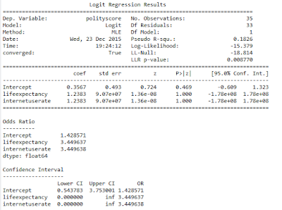
Test for Confounding

A logistic regression was run Internet Use Rate as explanatory variable with controlled variable Life expectancy.

The parameter values shows neither Internet Use rate nor Life expectancy is significant after controlling each in the logistic regression. In fact the relationship is non existent.

Test Multiple Regression

I am using Gapminder data set. My hypothesis is Life Expectancy is associated with Urban population rate in a positive way. Life expectancy is the response variable and Urban Population rate is the explanatory variable. I will be testing if any confounding exists with variables – income per person, employment rate, co2 emission and alcohol consumption

Code

# -*- coding: utf-8 -*-
"""
Created on Sat Dec 12 14:11:38 2015

@author: Abhishek
"""

import numpy
import pandas
import matplotlib.pyplot as plt
import statsmodels.api as sm
import statsmodels.formula.api as smf
import seaborn

# bug fix for display formats to avoid run time errors
pandas.set_option('display.float_format', lambda x:'%.2f'%x)

data = pandas.read_csv('gapminder.csv')

# convert to numeric format

# Response Variable
data['lifeexpectancy'] = pandas.to_numeric(data['lifeexpectancy'], errors='coerce')

# Explanatory Variables
data['urbanrate'] = pandas.to_numeric(data['urbanrate'], errors='coerce')
data['incomeperperson'] = pandas.to_numeric(data['incomeperperson'], errors='coerce')
data['employrate'] = pandas.to_numeric(data['employrate'], errors='coerce')
data['co2emissions'] = pandas.to_numeric(data['co2emissions'], errors='coerce')
data['alcconsumption'] = pandas.to_numeric(data['alcconsumption'], errors='coerce')

# listwise deletion of missing values
sub1 = data[['lifeexpectancy', 'urbanrate','incomeperperson','employrate','co2emissions','alcconsumption']].dropna()

# first order (linear) scatterplot
scat1 = seaborn.regplot(x="urbanrate", y="lifeexpectancy", scatter=True, data=sub1)
plt.xlabel('Urban Population Rate')
plt.ylabel('Life Expectancy')

# fit second order polynomial
# run the 2 scatterplots together to get both linear and second order fit lines
scat1 = seaborn.regplot(x="urbanrate", y="lifeexpectancy", scatter=True, order=2, data=sub1)
plt.xlabel('Urban Population Rate')
plt.ylabel('Life Expectancy')

# center quantitative IVs for regression analysis
sub1['urbanrate_c'] = (sub1['urbanrate'] - sub1['urbanrate'].mean())
sub1['incomeperperson_c'] = (sub1['incomeperperson'] - sub1['incomeperperson'].mean())
sub1['employrate_c'] = (sub1['employrate'] - sub1['employrate'].mean())
sub1['co2emissions_c'] = (sub1['co2emissions'] - sub1['co2emissions'].mean())
sub1['alcconsumption_c'] = (sub1['alcconsumption'] - sub1['alcconsumption'].mean())

# linear regression analysis
reg1 = smf.ols('lifeexpectancy ~ urbanrate_c', data=sub1).fit()
print (reg1.summary())

reg2 = smf.ols('lifeexpectancy ~ urbanrate_c  + incomeperperson_c + employrate_c + co2emissions_c + alcconsumption_c ', data=sub1).fit()
print (reg2.summary())

reg3 = smf.ols('lifeexpectancy ~ urbanrate_c + I(urbanrate_c**2) + employrate_c', data=sub1).fit()
print (reg3.summary())

#Q-Q plot for normality
fig4=sm.qqplot(reg1.resid, line='r')


# simple plot of residuals
stdres=pandas.DataFrame(reg1.resid_pearson)
plt.plot(stdres, 'o', ls='None')
l = plt.axhline(y=0, color='r')
plt.ylabel('Standardized Residual')
plt.xlabel('Observation Number')


# additional regression diagnostic plots
fig2 = plt.figure(figsize(10,5))
fig2 = sm.graphics.plot_regress_exog(reg3,  "employrate_c", fig=fig2)

# leverage plot
fig3=sm.graphics.influence_plot(reg3, size=8)
print(fig3)

Results

From the p value and coefficient it seems like there is strong linear relationship between life expectancy and urban population rate. A quadratic or higher order variable is not required in the regression test. The code above does show the second variable added to the OLS regression function for academic purpose only. Further test with other explanatory variable are conducted to test for confounding.

 R squared value: We did not find any confounding variables but controlling other variables in the OLS regression does increase the R square value. Which means, with more variables in the mix the variability in association between Life Expectancy and Urban Population rate is less

The q-q plot somewhat follows a straight line but deviates considerably at lower and higher quantiles. There could be other explanatory variables that might strengthen the association between life expectancy and urban population rate.

Most of the residuals in the above graph fall between one standard deviation of the mean, between -1 and 1. Visually we can ascertain that about 95% of the residuals falls between 2 standard deviation of the mean. Since there are residual values beyond 2 standard deviation of mean on either side, it is warning that there are outliers and model is not a great fit.

Test a Basic Linear Regression Model

I am testing the basic linear regression between Life Expectancy and Urban population rate. Data set used is Gapminder.

Code

# -*- coding: utf-8 -*-
"""
Created on Sun Dec  6 17:52:02 2015

@author: Abhishek
"""
import pandas
import statsmodels.formula.api as smf 
import seaborn
import matplotlib.pyplot as plt

# bug fix for display formats to avoid run time errors
pandas.set_option('display.float_format', lambda x:'%.2f'%x)

#call in data set
data = pandas.read_csv('gapminder.csv')

# convert variables to numeric format using convert_objects function
data['lifeexpectancy'] = pandas.to_numeric(data['lifeexpectancy'],errors='coerce')
data['urbanrate'] = pandas.to_numeric(data['urbanrate'],errors='coerce')

scat1 = seaborn.regplot(x="urbanrate", y="lifeexpectancy", scatter=True, data=data)
plt.ylabel('Life Expectancy')
plt.xlabel('Urbanization Rate')
plt.title ('Scatterplot for the Association Between Urban Rate and Life Expectancy')
print(scat1)

print ("OLS regression model for the association between urban rate and life expectancy")
# Quantitative Response Variable ~ Quantitative Explanatory Variable
reg1 = smf.ols('lifeexpectancy ~ urbanrate', data=data).fit()
print (reg1.summary())

Results

From above results - 

Dep Variable: Lifeexpectancy. This is the response variable. 

No. Observations: 188. Number of observations included in the analysis

F-statistic is 115.4 and p value is significantly smaller than alpha. This shows that we can safely reject null hypothesis.

Looking at the parameter estimates we can construct the life of best fir as follows - 

lifeexpectancy = 55.1732 + 0.2579 * urbanrate

P value from the P > |t| column can be reported as p < 0.0001. The values is very small, it is the value that would be obtained from Pearson Correlation Coefficient.

R-sqaured value: 0.38, accounts for 38% variability of response variable lifeexpectancy.