Test a Basic Linear Regression Model

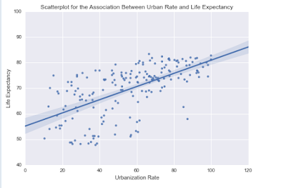
I am testing the basic linear regression between Life Expectancy and Urban population rate. Data set used is Gapminder.

Code

# -*- coding: utf-8 -*-
"""
Created on Sun Dec  6 17:52:02 2015

@author: Abhishek
"""
import pandas
import statsmodels.formula.api as smf 
import seaborn
import matplotlib.pyplot as plt

# bug fix for display formats to avoid run time errors
pandas.set_option('display.float_format', lambda x:'%.2f'%x)

#call in data set
data = pandas.read_csv('gapminder.csv')

# convert variables to numeric format using convert_objects function
data['lifeexpectancy'] = pandas.to_numeric(data['lifeexpectancy'],errors='coerce')
data['urbanrate'] = pandas.to_numeric(data['urbanrate'],errors='coerce')

scat1 = seaborn.regplot(x="urbanrate", y="lifeexpectancy", scatter=True, data=data)
plt.ylabel('Life Expectancy')
plt.xlabel('Urbanization Rate')
plt.title ('Scatterplot for the Association Between Urban Rate and Life Expectancy')
print(scat1)

print ("OLS regression model for the association between urban rate and life expectancy")
# Quantitative Response Variable ~ Quantitative Explanatory Variable
reg1 = smf.ols('lifeexpectancy ~ urbanrate', data=data).fit()
print (reg1.summary())

Results

From above results - 

Dep Variable: Lifeexpectancy. This is the response variable. 

No. Observations: 188. Number of observations included in the analysis

F-statistic is 115.4 and p value is significantly smaller than alpha. This shows that we can safely reject null hypothesis.

Looking at the parameter estimates we can construct the life of best fir as follows - 

lifeexpectancy = 55.1732 + 0.2579 * urbanrate

P value from the P > |t| column can be reported as p < 0.0001. The values is very small, it is the value that would be obtained from Pearson Correlation Coefficient.

R-sqaured value: 0.38, accounts for 38% variability of response variable lifeexpectancy.